
Synthesizing model metamers for TorchVision / TIMM models#
timm and torchvision are two model zoos from the deep learning community that contain many different models which one can use with plenoptic!
Warning
The following requires you to install torchvision and/or timm in your virtual environment, which can be done with pip.
import plenoptic as po
import torch
# needed for the plotting/animating:
%matplotlib inline
import matplotlib.pyplot as plt
plt.rcParams['animation.html'] = 'html5'
# use single-threaded ffmpeg for animation writer
plt.rcParams['animation.writer'] = 'ffmpeg'
plt.rcParams['animation.ffmpeg_args'] = ['-threads', '1']
DEVICE = torch.device('cuda' if torch.cuda.is_available() else 'cpu')
import torchvision
from torchvision.models import feature_extraction
import numpy as np
When synthesizing model metamers for convolutional neural networks, researchers often pick a specific layer whose output they want to match (e.g., Feather et al., 2023).
torchvision contains a “feature extractor” which we can use to grab the activation from a specific layer for most pytorch models, and we can use a small wrapper to handle this for us (this class will eventually be part of plenoptic – in a release probably later this summer). In the following (large!) block of code, only the __init__ and forward are necessary. However, defining plot_representation method in this way allows us to make use of the built-in plot_synthesis_status and animate functions we used in some of the other notebooks!
class TorchVisionModel(torch.nn.Module):
    def __init__(self, model, return_node, transform=None):
        super().__init__()
        self.transform = transform
        self.extractor = feature_extraction.create_feature_extractor(model, [return_node])
        self.model = model
        self.return_node = return_node

    def forward(self, x):
        if self.transform is not None:
            x = self.transform(x)
        return self.extractor(x)[self.return_node]

    def plot_representation(
        self,
        data: torch.Tensor,
        ax = None,
        figsize = (15, 15),
        ylim = None,
        batch_idx = 0,
        title = None,
    ):
        # Select the batch index
        data = data[batch_idx]

        # Compute across channels spatal error
        spatial_error = torch.abs(data).mean(dim=0).detach().cpu().numpy()

        # Compute per-channel error
        error = torch.abs(data).mean(dim=(1, 2))  # Shape: (C,)
        sorted_idx = torch.argsort(error, descending=True)
        sorted_error = error[sorted_idx].detach().cpu().numpy()

        # Determine figure layout
        if ax is None:
            fig, axes = plt.subplots(2, 1, figsize=figsize, gridspec_kw={"height_ratios": [1, 1]})
        else:
            ax = po.tools.clean_up_axes(ax, False, ["top", "right", "bottom", "left"], ["x", "y"])
            gs = ax.get_subplotspec().subgridspec(2, 1, height_ratios=[3, 1])
            fig = ax.figure
            axes = [fig.add_subplot(gs[0]), fig.add_subplot(gs[1])]

        # Plot average error across channels
        po.imshow(
            ax=axes[0], image=spatial_error[None, None, ...], title="Average Error Across Channels", vrange="auto0"
        )
        # axes[0].set_title()

        # Plot channel error distribution
        x_pos = np.arange(20)
        axes[1].bar(x_pos, sorted_error[:20], color="C1", alpha=0.7)
        axes[1].set_xticks(x_pos)
        axes[1].set_xticklabels(sorted_idx[:20].tolist(), rotation=45)
        axes[1].set_xlabel("Channel")
        axes[1].set_ylabel("Absolute error")
        axes[1].set_title("Top 20 Channels Contributions to Error")

        if title is not None:
            fig.suptitle(title)

        return fig, axes
Use a model from torchvision#
Torchvision models are found within torchvision.models and are often represented in the following fashion:
weights = torchvision.models.ResNet50_Weights.IMAGENET1K_V1
model = torchvision.models.resnet50(weights=weights)
Downloading: "https://download.pytorch.org/models/resnet50-0676ba61.pth" to /home/agent/workspace/neurorse_plenoptic-vss-2025_main/.cache/torch/hub/checkpoints/resnet50-0676ba61.pth
0%| | 0.00/97.8M [00:00<?, ?B/s]
25%|██▍ | 24.1M/97.8M [00:00<00:00, 253MB/s]
50%|█████ | 49.1M/97.8M [00:00<00:00, 258MB/s]
76%|███████▌ | 74.1M/97.8M [00:00<00:00, 260MB/s]
100%|██████████| 97.8M/97.8M [00:00<00:00, 260MB/s]
Additionally, many deep net models have an associated preprocessing transform, which depends on the dataset they were trained upon. For ImageNet-trained models, they will generally downsample and crop their images to be 224 x 224, and then normalize the RGB values. My recommendation is to include the normalization within the model (as far as plenoptic is concerned), while the resizing of the image is handled outside. In torchvision, both of these steps are bundled together in the transforms class:
transform = weights.transforms()
transform
ImageClassification(
    crop_size=[224]
    resize_size=[256]
    mean=[0.485, 0.456, 0.406]
    std=[0.229, 0.224, 0.225]
    interpolation=InterpolationMode.BILINEAR
)
The above transformation will always resize an image to 256 x 256 and then crop out the center 224 x 224 pixels (even if you pass it an image that’s 224 x 224!). I have not yet figured out a way to “split up” this transform (separating out the normalization) or otherwise disabling the resizing, so let’s manually create a Normalize transform with the right means and stds:
norm = torchvision.transforms.Normalize(transform.mean, transform.std)
There’s one more step we need: we need to decide which layer’s output we wish to examine. Torchvision has a helper function for finding layer names (it returns two lists, one for train mode, one for eval; we want the eval):
feature_extraction.get_graph_node_names(model)[1]
['x',
 'conv1',
 'bn1',
 'relu',
 'maxpool',
 'layer1.0.conv1',
 'layer1.0.bn1',
 'layer1.0.relu',
 'layer1.0.conv2',
 'layer1.0.bn2',
 'layer1.0.relu_1',
 'layer1.0.conv3',
 'layer1.0.bn3',
 'layer1.0.downsample.0',
 'layer1.0.downsample.1',
 'layer1.0.add',
 'layer1.0.relu_2',
 'layer1.1.conv1',
 'layer1.1.bn1',
 'layer1.1.relu',
 'layer1.1.conv2',
 'layer1.1.bn2',
 'layer1.1.relu_1',
 'layer1.1.conv3',
 'layer1.1.bn3',
 'layer1.1.add',
 'layer1.1.relu_2',
 'layer1.2.conv1',
 'layer1.2.bn1',
 'layer1.2.relu',
 'layer1.2.conv2',
 'layer1.2.bn2',
 'layer1.2.relu_1',
 'layer1.2.conv3',
 'layer1.2.bn3',
 'layer1.2.add',
 'layer1.2.relu_2',
 'layer2.0.conv1',
 'layer2.0.bn1',
 'layer2.0.relu',
 'layer2.0.conv2',
 'layer2.0.bn2',
 'layer2.0.relu_1',
 'layer2.0.conv3',
 'layer2.0.bn3',
 'layer2.0.downsample.0',
 'layer2.0.downsample.1',
 'layer2.0.add',
 'layer2.0.relu_2',
 'layer2.1.conv1',
 'layer2.1.bn1',
 'layer2.1.relu',
 'layer2.1.conv2',
 'layer2.1.bn2',
 'layer2.1.relu_1',
 'layer2.1.conv3',
 'layer2.1.bn3',
 'layer2.1.add',
 'layer2.1.relu_2',
 'layer2.2.conv1',
 'layer2.2.bn1',
 'layer2.2.relu',
 'layer2.2.conv2',
 'layer2.2.bn2',
 'layer2.2.relu_1',
 'layer2.2.conv3',
 'layer2.2.bn3',
 'layer2.2.add',
 'layer2.2.relu_2',
 'layer2.3.conv1',
 'layer2.3.bn1',
 'layer2.3.relu',
 'layer2.3.conv2',
 'layer2.3.bn2',
 'layer2.3.relu_1',
 'layer2.3.conv3',
 'layer2.3.bn3',
 'layer2.3.add',
 'layer2.3.relu_2',
 'layer3.0.conv1',
 'layer3.0.bn1',
 'layer3.0.relu',
 'layer3.0.conv2',
 'layer3.0.bn2',
 'layer3.0.relu_1',
 'layer3.0.conv3',
 'layer3.0.bn3',
 'layer3.0.downsample.0',
 'layer3.0.downsample.1',
 'layer3.0.add',
 'layer3.0.relu_2',
 'layer3.1.conv1',
 'layer3.1.bn1',
 'layer3.1.relu',
 'layer3.1.conv2',
 'layer3.1.bn2',
 'layer3.1.relu_1',
 'layer3.1.conv3',
 'layer3.1.bn3',
 'layer3.1.add',
 'layer3.1.relu_2',
 'layer3.2.conv1',
 'layer3.2.bn1',
 'layer3.2.relu',
 'layer3.2.conv2',
 'layer3.2.bn2',
 'layer3.2.relu_1',
 'layer3.2.conv3',
 'layer3.2.bn3',
 'layer3.2.add',
 'layer3.2.relu_2',
 'layer3.3.conv1',
 'layer3.3.bn1',
 'layer3.3.relu',
 'layer3.3.conv2',
 'layer3.3.bn2',
 'layer3.3.relu_1',
 'layer3.3.conv3',
 'layer3.3.bn3',
 'layer3.3.add',
 'layer3.3.relu_2',
 'layer3.4.conv1',
 'layer3.4.bn1',
 'layer3.4.relu',
 'layer3.4.conv2',
 'layer3.4.bn2',
 'layer3.4.relu_1',
 'layer3.4.conv3',
 'layer3.4.bn3',
 'layer3.4.add',
 'layer3.4.relu_2',
 'layer3.5.conv1',
 'layer3.5.bn1',
 'layer3.5.relu',
 'layer3.5.conv2',
 'layer3.5.bn2',
 'layer3.5.relu_1',
 'layer3.5.conv3',
 'layer3.5.bn3',
 'layer3.5.add',
 'layer3.5.relu_2',
 'layer4.0.conv1',
 'layer4.0.bn1',
 'layer4.0.relu',
 'layer4.0.conv2',
 'layer4.0.bn2',
 'layer4.0.relu_1',
 'layer4.0.conv3',
 'layer4.0.bn3',
 'layer4.0.downsample.0',
 'layer4.0.downsample.1',
 'layer4.0.add',
 'layer4.0.relu_2',
 'layer4.1.conv1',
 'layer4.1.bn1',
 'layer4.1.relu',
 'layer4.1.conv2',
 'layer4.1.bn2',
 'layer4.1.relu_1',
 'layer4.1.conv3',
 'layer4.1.bn3',
 'layer4.1.add',
 'layer4.1.relu_2',
 'layer4.2.conv1',
 'layer4.2.bn1',
 'layer4.2.relu',
 'layer4.2.conv2',
 'layer4.2.bn2',
 'layer4.2.relu_1',
 'layer4.2.conv3',
 'layer4.2.bn3',
 'layer4.2.add',
 'layer4.2.relu_2',
 'avgpool',
 'flatten',
 'fc']
So let’s pick one of those and put it all together:
model = TorchVisionModel(model, "layer2", norm)
Synthesize model metamers!#
Now we can use the above like any other model we’ve used so far, with one note: these models expect RGB images
img = po.data.einstein(as_gray=False).to(DEVICE)
model.to(DEVICE)
po.tools.remove_grad(model)
model.eval()
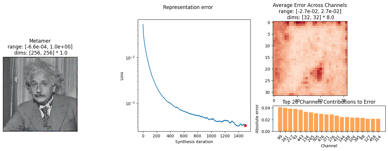
met = po.synth.Metamer(img, model)
met.synthesize(max_iter=1500, stop_criterion=1e-11, store_progress=10)
po.synth.metamer.plot_synthesis_status(met, ylim=False)
Clipping input data to the valid range for imshow with RGB data ([0..1] for floats or [0..255] for integers). Got range [-0.0006586362..0.9999923].
(<Figure size 1700x500 with 5 Axes>,
 {'display_metamer': 0,
  'plot_loss': 1,
  'plot_representation_error': [3, 4, 2],
  'misc': []})
Use a model from timm#
timm models operate in much the same way as torchvision, though with a slightly different syntax for creation of the model and transform:
import timm
from timm.data import resolve_data_config
from timm.data.transforms_factory import create_transform

model = timm.create_model("hf-hub:nateraw/resnet50-oxford-iiit-pet", pretrained=True)
# Create Transform
transform = create_transform(**resolve_data_config(model.pretrained_cfg, model=model))
This model has the same resizing / cropping transform as above, but timm represents their transform in a way that allows us to select the steps we want, so we can more straightforwardly just grab the normalization one:
print(transform)
transform = transform.transforms[-1]
transform
Compose(
    Resize(size=235, interpolation=bicubic, max_size=None, antialias=True)
    CenterCrop(size=(224, 224))
    MaybeToTensor()
    Normalize(mean=tensor([0.4850, 0.4560, 0.4060]), std=tensor([0.2290, 0.2240, 0.2250]))
)
Normalize(mean=tensor([0.4850, 0.4560, 0.4060]), std=tensor([0.2290, 0.2240, 0.2250]))
And similarly, we have to choose a specific layer. We can see their names with the same helper function as above. But let’s just grab the same layer:
model = TorchVisionModel(model, "layer2", norm)